Parallel Monto-Carlo options pricing

This notebook shows how to use ipyparallel to do Monte-Carlo options pricing in parallel. We will compute the price of a large number of options for different strike prices and volatilities.

Problem setup

%matplotlib inline
import matplotlib.pyplot as plt

import numpy as np

Here are the basic parameters for our computation.

price = 100.0  # Initial price
rate = 0.05  # Interest rate
days = 260  # Days to expiration
paths = 10000  # Number of MC paths
n_strikes = 6  # Number of strike values
min_strike = 90.0  # Min strike price
max_strike = 110.0  # Max strike price
n_sigmas = 5  # Number of volatility values
min_sigma = 0.1  # Min volatility
max_sigma = 0.4  # Max volatility

strike_vals = np.linspace(min_strike, max_strike, n_strikes)
sigma_vals = np.linspace(min_sigma, max_sigma, n_sigmas)

print("Strike prices: ", strike_vals)
print("Volatilities: ", sigma_vals)

Strike prices:  [ 90.  94.  98. 102. 106. 110.]
Volatilities:  [0.1   0.175 0.25  0.325 0.4  ]

Monte-Carlo option pricing function

The following function computes the price of a single option. It returns the call and put prices for both European and Asian style options.

def price_option(S=100.0, K=100.0, sigma=0.25, r=0.05, days=260, paths=10000):
    """
    Price European and Asian options using a Monte Carlo method.

    Parameters
    ----------
    S : float
        The initial price of the stock.
    K : float
        The strike price of the option.
    sigma : float
        The volatility of the stock.
    r : float
        The risk free interest rate.
    days : int
        The number of days until the option expires.
    paths : int
        The number of Monte Carlo paths used to price the option.

    Returns
    -------
    A tuple of (E. call, E. put, A. call, A. put) option prices.
    """
    from math import exp, sqrt

    import numpy as np

    h = 1.0 / days
    const1 = exp((r - 0.5 * sigma**2) * h)
    const2 = sigma * sqrt(h)
    stock_price = S * np.ones(paths, dtype='float64')
    stock_price_sum = np.zeros(paths, dtype='float64')
    for j in range(days):
        growth_factor = const1 * np.exp(const2 * np.random.standard_normal(paths))
        stock_price = stock_price * growth_factor
        stock_price_sum = stock_price_sum + stock_price
    stock_price_avg = stock_price_sum / days
    zeros = np.zeros(paths, dtype='float64')
    r_factor = exp(-r * h * days)
    euro_put = r_factor * np.mean(np.maximum(zeros, K - stock_price))
    asian_put = r_factor * np.mean(np.maximum(zeros, K - stock_price_avg))
    euro_call = r_factor * np.mean(np.maximum(zeros, stock_price - K))
    asian_call = r_factor * np.mean(np.maximum(zeros, stock_price_avg - K))
    return (euro_call, euro_put, asian_call, asian_put)

We can time a single call of this function using the %timeit magic:

%time result = price_option(S=100.0, K=100.0, sigma=0.25, r=0.05, days=260, paths=10000)
result  # noqa

CPU times: user 75.9 ms, sys: 9.47 ms, total: 85.4 ms
Wall time: 90.6 ms

(np.float64(12.292386227996472),
 np.float64(7.565358135751658),
 np.float64(6.843004428201171),
 np.float64(4.4762283778996155))

Parallel computation across strike prices and volatilities

The Client is used to setup the calculation and works with all engines.

import ipyparallel as ipp

rc = ipp.Cluster().start_and_connect_sync()

Starting 10 engines with <class 'ipyparallel.cluster.launcher.LocalEngineSetLauncher'>

A LoadBalancedView is an interface to the engines that provides dynamic load balancing at the expense of not knowing which engine will execute the code.

view = rc.load_balanced_view()

Submit tasks for each (strike, sigma) pair. Again, we use the %%timeit magic to time the entire computation.

async_results = []

%%time

for strike in strike_vals:
    for sigma in sigma_vals:
        # This line submits the tasks for parallel computation.
        ar = view.apply_async(price_option, price, strike, sigma, rate, days, paths)
        async_results.append(ar)

rc.wait(async_results)  # Wait until all tasks are done.

CPU times: user 38.4 ms, sys: 12.1 ms, total: 50.5 ms
Wall time: 348 ms

True

len(async_results)

30

Process and visualize results

Retrieve the results using the get method:

results = [ar.get() for ar in async_results]

Assemble the result into a structured NumPy array.

prices = np.empty(
    n_strikes * n_sigmas,
    dtype=[('ecall', float), ('eput', float), ('acall', float), ('aput', float)],
)

for i, price in enumerate(results):
    prices[i] = tuple(price)

prices.shape = (n_strikes, n_sigmas)

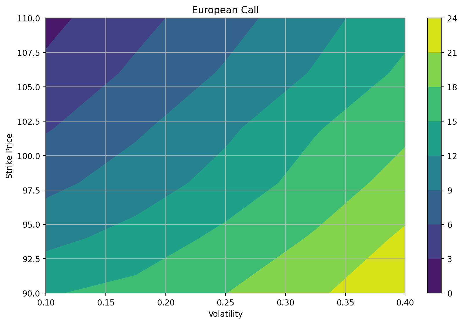
Plot the value of the European call in (volatility, strike) space.

plt.figure()
plt.contourf(sigma_vals, strike_vals, prices['ecall'])
plt.axis('tight')
plt.colorbar()
plt.title('European Call')
plt.xlabel("Volatility")
plt.ylabel("Strike Price")

Text(0, 0.5, 'Strike Price')

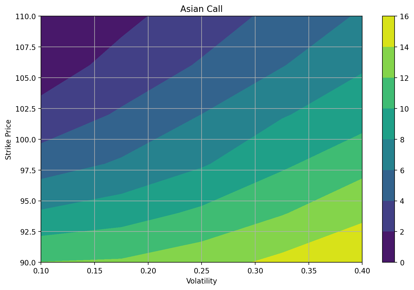
Plot the value of the Asian call in (volatility, strike) space.

plt.figure()
plt.contourf(sigma_vals, strike_vals, prices['acall'])
plt.axis('tight')
plt.colorbar()
plt.title("Asian Call")
plt.xlabel("Volatility")
plt.ylabel("Strike Price")

Text(0, 0.5, 'Strike Price')

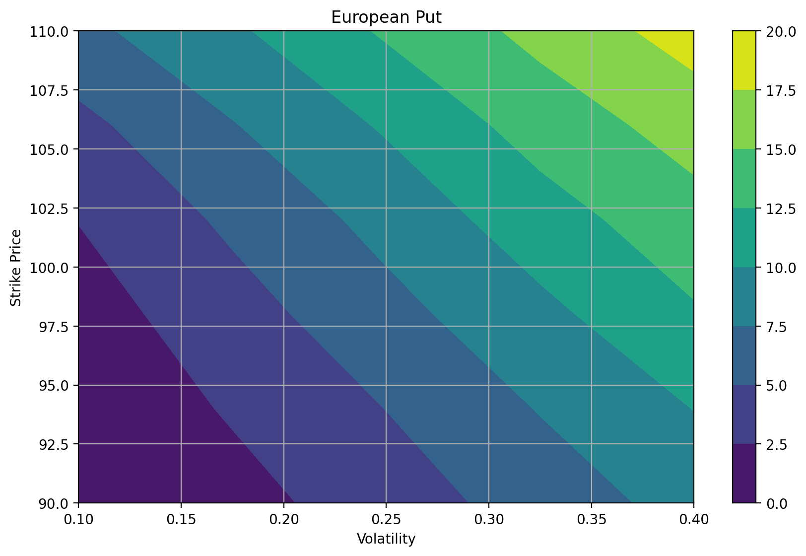
Plot the value of the European put in (volatility, strike) space.

plt.figure()
plt.contourf(sigma_vals, strike_vals, prices['eput'])
plt.axis('tight')
plt.colorbar()
plt.title("European Put")
plt.xlabel("Volatility")
plt.ylabel("Strike Price")

Text(0, 0.5, 'Strike Price')

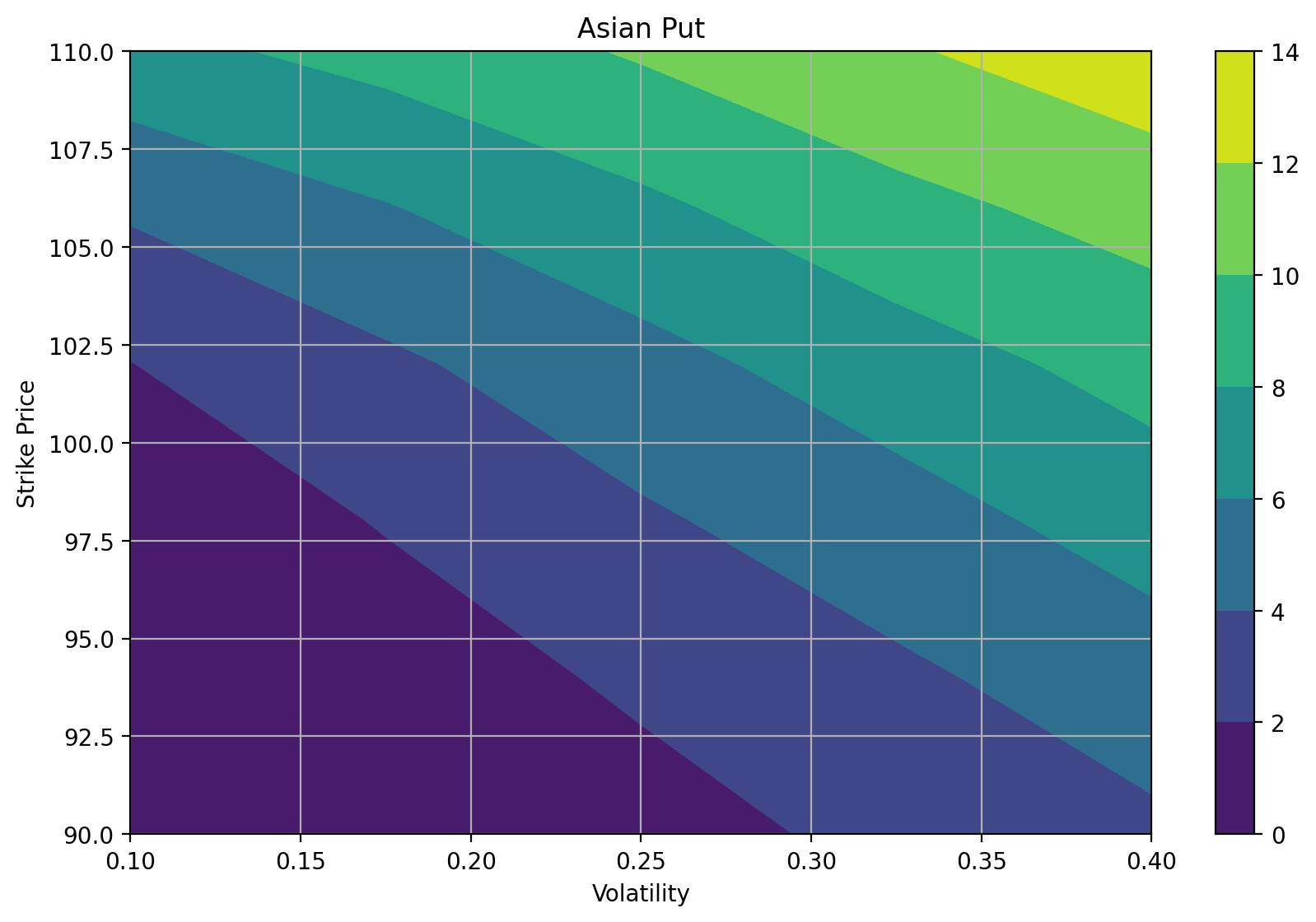
Plot the value of the Asian put in (volatility, strike) space.

plt.figure()
plt.contourf(sigma_vals, strike_vals, prices['aput'])
plt.axis('tight')
plt.colorbar()
plt.title("Asian Put")
plt.xlabel("Volatility")
plt.ylabel("Strike Price")

Text(0, 0.5, 'Strike Price')